Category: Uncategorized

  • Case study: R (tidyverse) vs Python (pandas)

    Case study: R (tidyverse) vs Python (pandas)

    The problem

    An old friend e-mailed me a challenge today. He was working with a data file which contains measurements of compounds from groundwater taps. The file looks like this (when opened in a spreadsheet program):

    In other words, it contains measurements for a particular date for a particular tap point and compound.

    He was using the following R code to plot how the Iron levels varied over time at different sampling points:

    library(tidyverse)
    
    ggplot(data) +
      geom_line(mapping = aes(x=Date,y=Tap4.Fe,color="red")) +
      geom_line(mapping = aes(x=Date,y=Tap5.Fe,color="blue")) +
      geom_line(mapping = aes(x=Date,y=Tap6.Fe,color="purple")) +
      geom_line(mapping = aes(x=Date,y=Tap7.Fe,color="green")) +
      geom_line(mapping = aes(x=Date,y=Tap8.Fe,color="orange")) +
      geom_line(mapping = aes(x=Date,y=Tap9.Fe,color="brown"))


    But he could sense that this was not an optimal solution to the problem and wanted some advice on getting this to work better.

    Tidy data

    My first comment to him was that this data is not in the format which the tidyverse wants. Hadley Wickham appears to have revitalised the R language with his clever packages and wrote a manifesto of sorts to the benefits of tidy data, which I feel is really just a no-nonsense approach to data normalisation. There are many things wrong with the data in its current form, but I see spreadsheets like this quite often.
    The problem is that people want an easy way of entering data and often end up focusing on ease of entry instead of ease of analysis. It is easy to understand how this format grows by adding more readings as extra columns on the spreadsheet and having one date per row. 
    From a normalisation perspective, the problems with this format are that there is data in the column name: Tap4.Fe is actually encoding two fields – a position and a compound. Our first job is therefore to tidy up this data.
    The tidyverse supplies a lot of useful functions to do just that. Here is how I tidied the data:
    measurements %
      gather(measurement, value, -Date) %>% 
      separate(measurement, c(“position”, “compound”), sep=”\.”) %>%
      drop_na()
    Now measurements is much “taller” and less wide:

    The key points here are that we have a single row for a single observation. This is the essence of the tidy data philosophy and it makes downstream processing very easy.

    Here is how I recreated his plots:

    filter(measurements, compound == “Fe”) %>% 
      ggplot + 
      aes(x = Date, y = value, color = position) + geom_line()

    That’s really nice. I can filter to find the Iron measurements and I can have ggplot handle the colours automatically by looking at the position.

    The resulting plot looks like this (this is just with all default settings):

    Python

    I was very happy with how succinct the R version of the solution was, but I use Python more than R, so I was interested to see how Pandas handles this.
    The “tidyfication” of the data requires a lot more ceremony in Pandas:
    df = (pandas.read_csv(‘data.csv’, parse_dates=[‘Date’])
          .melt(id_vars=’Date’)
          .dropna())
    df[[‘position’, ‘compound’]] = df.variable.str.split(‘.’, expand=True)
    del df[‘variable’]
    I’m especially critical of how hard it is to replace a compound column with its split version (the last two lines). Wickham clearly understands that this is a common problem in data files, where the Pandas version feels “hacky”.
    Now the code to recreate the graphics:
    df.query(‘compound==”Fe”‘).pivot(index=’Date’, columns=’position’, values=’value’).plot()
    Again, I am using the default settings. Although that might look a bit simpler than the R code, it took me ages to write. There is a bit of counter-intuitive (to my mind) pivoting so that I can use the built-in Pandas plot command and I have much less flexibility about the mapping.
    I suppose the take-home here is that tidying your data is a win regardless of your platform, but that R and the tidyverse is really a force to be reckoned with. I’m hoping the Pandas API will end up providing some of the powerful verbs from tidyr et al eventually.
  • My programming history (part 2)

    This post overlaps a little bit with the the previous one, recapping my programming history.

    We ended the previous part in 2002 when I finished my Masters and started teaching, but I want to go into a little more detail on my history with scripting languages.

    I encountered Matlab for the first time in my second year (in 1998) in a course called CRV220. I still have the study guide so I can say with confidence that we were taught a combination of Turbo Pascal and Matlab. At the time, the Turbo Pascal environment was much nicer than the Matlab one. Even though the Borland IDE was text-based, it had syntax highlighting and step-by-step debugging. It looked like this:

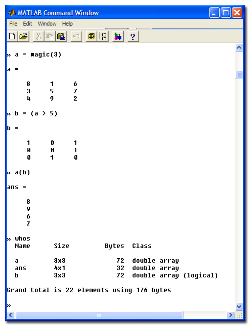
    By contrast, in 1998 Matlab was in version 5.2 and looked like this:

    We typed Matlab code into Notepad and executed it from this command window. The most impressive part of Matlab was that it could produce graphical output very easily. But the development environment was non-existent. It was, however, very clear that you could solve engineering problems using much less Matlab code than Turbo Pascal. Matlab was also the first language I encountered which had a REPL – you could type commands into the command window one at a time and see the result. I really liked this concept.

    In 1998 also bought an HP 48 GL calculator and spent a lot of time programming it do solve problems like balancing chemical equations and so on. We were often allowed to use our calculators in tests, but they were often cleared before we wrote. The HP introduced me to the idea of stack-based languages.

    In my final year (in 2000), we did our final year project calculations using a spreadsheet called Quattro Pro, since Excel had not yet achieved the dominant position it currently enjoys. We did not do much programming in our final year.

    By the time I started my Masters in 2001, Matlab had just undergone a major rework in the release of version 6, moving to a Java-based workspace and for the first time Matlab was an IDE with an integrated code editor, debugging, and all the features from the Turbo Pascal IDE that I had missed when I first encountered Matlab. I found this new environment quite comfortable and used it happily throughout my Masters work. I used it to do the actual simulation and to produce all the graphs in my dissertation. But I had also bumped up against one of the things that Matlab was not very good at when I was writing the code to make the call graph I posted in the previous part: Matlab was really terrible at text processing.

    By 2002 I was completely immersing myself in the Unix way. I had started to see the power of the “small tools doing one thing well” philosophy and spend a great deal of time reading the GNU Info pages for all the various unix tools while also learning about Richard Stalman and the Free Software movement. I was using Matlab on my Linux machine and learning bash. This is when I started learning Emacs, after reading In the beginning was the commandline where Neal Stephenson says the following about it:

    “I use emacs, which might be thought of as a thermonuclear word processor. It was created by Richard Stallman; enough said. It is written in Lisp, which is the only computer language that is beautiful. It is colossal, and yet it only edits straight ASCII text files, which is to say, no fonts, no boldface, no underlining. In other words, the engineer-hours that, in the case of Microsoft Word, were devoted to features like mail merge, and the ability to embed feature-length motion pictures in corporate memoranda, were, in the case of emacs, focused with maniacal intensity on the deceptively simple-seeming problem of editing text.”

    Teaching

    In the first semester of 2002 I was the teaching assistant for CRV210 (the same subject where I had learned Matlab, now moved to the first semester). In the second semester I took over CMO320 (Mass transfer) from a lecturer who had moved to New Zealand. At this point I was done with my Masters and thinking of but had not yet enrolled for my PhD. I barely kept my head above water in that first semester, having to revise the material even as I taught it. In the second go around I started using more computer methods in my teaching, using Excel and Matlab to solve mass transfer problems.

    As I did this, I started realising that our students were not well prepared to deal with computer solutions of these problems. I eventually moved over to teaching our computer course.

    Other languages

    I started evaluating different scripting languages which would be better at the kinds of string processing I had done for the call graph program and came across Perl and Python around this time. The earliest proper Python program I could find in my records was from 2004 and was for creating the same kind of file I used to do the call graph (the GraphViz package). I also learned the classic grep, sed and awk combination for text processing in Linux, motivated largely by reading “Unix Text Processing

    I picked up Fortran around 2005 as I started looking for ways to speed up my simulations. In the process I learned that modern Fortran was not at all like the FORTRAN 77 that people love to mock. It is a pretty decent language for numerical work. I learned R in 2007 while I was looking for better ways to handle statistical graphics. At that time R was the best language to learn for statistical work. Some might say it still is, even though Python has the big momentum for data science as of 2017.

    Teaching programming

    I started teaching CRV210 in 2006. Before I did, I went on a deep dive to understand the best ways to teach programming. I found out about the MIT programming course and read The Structure and Interpretation of Computer Programs, picking up a deep and abiding love for Lisp in the process. I read up on SmallTalk, various graphical languages for teaching programming and all the different models which can be used to understand programming.

    I settled on teaching Matlab with a strong focus on functional programming. I taught students to avoid scripts and write everything as functions, building functionality up slowly. I taught recursion and scoping before I even handled basic iteration (for loops). I think this made students understand functions a lot better, but it was an unpopular choice. My students tend to view programming more as a necessary evil than the transformative experience I found it to be. They want to solve problems and learn as little programming on the way to those solutions. This made my course feel hopelessly obtuse as I went over problems like computability and logic before simple things like solving a set of equations using the tools.

    Moving from Matlab to open source and Python

    Not long after I started teaching programming, it became clear to me that students were pirating Matlab at an alarming rate. Part of the problem was that the cheap student version could only handle small matrices. The problem actually became more pronounced after the Mathworks moved over to a more capable student version which required you to send in your proof of registration to get the student discount. Most students found it easier to crack a downloaded version than to deal with the paperwork of getting the student version. The university was also paying a large sum of money to retain Matlab licenses for the lab computers, and we calculated large costs for he research license which we would need to do actual research with Matlab instead of only using it for teaching.

    I started gathering support for a move to Python. The first phase of this was to stop renewing our license for Matlab and move to Octave, an open-source reimplementation of  Matlab. This allowed lecturers to retain their Matlab code and get used to a less featureful environment (we were back to a single window interface). CRV was taught for the last time in 2008. Our students started attending the MPR212 classes in 2009, which are now still taught to all the engineering students at UP. They moved to Python in 2013 and from Python scripts to Jupyter Notebooks in 2016.

    The notebook revolution

    I started hearing about IPython notebooks around 2011, but I only started using them at the end of 2012. It took a while for me to warm to them, but I now feel they are excellent as an exploration tool as well as a teaching tool. I have committed deeply to producing notebooks for the subjects that I teach. There is a great deal of momentum behind the Jupyter project right now and I think they will continue to be one of the best ways to interact with your code for a couple of years yet. My one big issue with notebooks is that bundling the results of calculations together with the code makes it quite hard to handle them in source code management tools. But I am also sure that a future incarnation will fix this issue. It’s not a big enough problem to cancel the benefit.

    Final word

    Right now I feel like we made the right bet when we moved away from Matlab. Python is a much more general purpose language and has a large installed base. I think it is a better first language than Matlab and is something that you can see yourself using even when you go to industry. Of course Matlab hasn’t stood still, and is still one of the fastest ways to solve a problem if a toolbox exists for the field you’re in, but I haven’t felt the need to open much else than Python for a very long time.

    I’m keeping an eye on Julia as a competitor to Python in the computational space, but so far it seems to lack critical mass. I’m also testing the waters on Rust as a replacement for Fortran for my high speed code, but it also has too little support for the well-established numerical libraries.

    I think the last bit of my recap on history will be about simulation environments, moving from Simulink to Modelica, but this post is probably already too long.

  • A simple GUI spreadsheet in less than 100 lines of Python

    Original challenge: Standard library only

    I set myself a little challenge to write a simple spreadsheet-like program in Python in less than 100 lines, using only the standard library.

    The code in this repository manages it in 100 non-blank lines, including comments. 88 if you ignore the comments. The full code is also at the end of this post. Note: I have also redone the code in PyQT5. This is discussed after the tkinter code.

    This is what it the program looks like when you run it:

    You can click on cells to edit their formulae and move around with the arrow keys. Formulae are evaluated once you press Return or navigate way from a cell. Every cell is evaluated as a Python expression. This means you don’t do the Excel thing of having formulae start with =. Everything is a fomula. So the formula in A2 in the screenshot above is valid and will evaluate to 1 once focus moves away from the cell. The math module is imported by default, so you can use sin and cos and so on. I use a very cheap and nasty call of eval to make it all work, which you should never do for production code.

    Other than using eval, I also play a little fast and loose with the way objects are allowed to touch each other in the code. I allow each cell to access all their siblings directly instead of going through an intermediary. I probably also break a couple of other OO rules along the way with the way the cells propagate their calculations when they are changed. But the whole code only took a couple of hours to write and it actually works.

    And now, here is the full code:

    #!/usr/bin/env python
    
    import tkinter as tk
    import math
    import re
    from collections import ChainMap
    
    Nrows = 5
    Ncols = 5
    
    cellre = re.compile(r'b[A-Z][0-9]b')
    
    
    def cellname(i, j):
        return f'{chr(ord("A")+j)}{i+1}'
    
    
    class Cell():
        def __init__(self, i, j, siblings, parent):
            self.row = i
            self.col = j
            self.siblings = siblings
            self.name = cellname(i, j)
            self.formula = '0'
            self.value = 0
            # Dependencies - must be updated if this cell changes
            self.deps = set()
            # Requirements - values required for this cell to calculate
            self.reqs = set()
    
            self.var = tk.StringVar()
            entry = self.widget = tk.Entry(parent,
                                           textvariable=self.var,
                                           justify='right')
            entry.bind('<FocusIn>', self.edit)
            entry.bind('<FocusOut>', self.update)
            entry.bind('<Return>', self.update)
            entry.bind('<Up>', self.move(-1, 0))
            entry.bind('<Down>', self.move(+1, 0))
            entry.bind('<Left>', self.move(0, -1))
            entry.bind('<Right>', self.move(0, 1))
    
            self.var.set(self.value)
    
        def move(self, rowadvance, coladvance):
            targetrow = (self.row + rowadvance) % Nrows
            targetcol = (self.col + coladvance) % Ncols
    
            def focus(event):
                targetwidget = self.siblings[cellname(targetrow, targetcol)].widget
                targetwidget.focus()
    
            return focus
    
        def calculate(self):
            currentreqs = set(cellre.findall(self.formula))
    
            # Add this cell to the new requirement's dependents
            for r in currentreqs - self.reqs:
                self.siblings[r].deps.add(self.name)
            # Add remove this cell from dependents no longer referenced
            for r in self.reqs - currentreqs:
                self.siblings[r].deps.remove(self.name)
    
            # Look up the values of our required cells
            reqvalues = {r: self.siblings[r].value for r in currentreqs}
            # Build an environment with these values and basic math functions
            environment = ChainMap(math.__dict__, reqvalues)
            # Note that eval is DANGEROUS and should not be used in production
            self.value = eval(self.formula, {}, environment)
    
            self.reqs = currentreqs
            self.var.set(self.value)
    
        def propagate(self):
            for d in self.deps:
                self.siblings[d].calculate()
                self.siblings[d].propagate()
    
        def edit(self, event):
            self.var.set(self.formula)
            self.widget.select_range(0, tk.END)
    
        def update(self, event):
            self.formula = self.var.get()
            self.calculate()
            self.propagate()
            # If this was after pressing Return, keep showing the formula
            if hasattr(event, 'keysym') and event.keysym == "Return":
                self.var.set(self.formula)
    
    
    class SpreadSheet(tk.Frame):
        def __init__(self, rows, cols, master=None):
            super().__init__(master)
            self.rows = rows
            self.cols = cols
            self.cells = {}
    
            self.pack()
            self.create_widgets()
    
        def create_widgets(self):
            # Frame for all the cells
            self.cellframe = tk.Frame(self)
            self.cellframe.pack(side='top')
    
            # Column labels
            blank = tk.Label(self.cellframe)
            blank.grid(row=0, column=0)
            for j in range(self.cols):
                label = tk.Label(self.cellframe, text=chr(ord('A')+j))
                label.grid(row=0, column=j+1)
    
            # Fill in the rows
            for i in range(self.rows):
                rowlabel = tk.Label(self.cellframe, text=str(i + 1))
                rowlabel.grid(row=1+i, column=0)
                for j in range(self.cols):
                    cell = Cell(i, j, self.cells, self.cellframe)
                    self.cells[cell.name] = cell
                    cell.widget.grid(row=1+i, column=1+j)
    
    
    root = tk.Tk()
    app = SpreadSheet(Nrows, Ncols, master=root)
    app.mainloop()
    

    Part 2: PyQT5

    I posted this blog to Reddit and one of the commenters mentioned that PyQT5 has a nice table widget which is more spreadsheet-like. So I re-did the spreadsheet in PyQT5. The code is functionally similar at the moment and also has approximately the same number of lines (87 non-comment code lines). The main differences are that I could use the QTableWidget to handle all the navigation. I had to do some interesting things with delegates to enable to editing mode I wanted, though, which cost me all the lines I saved from the navigation. I think my next step is going to be to extract the calculation logic into a common class which both of these can use – there is way too much duplication going on here right now!

    So, this is what the PyQT5 one looks like. It’s a little more compact, but otherwise very similar. The interaction is slightly more spreadsheet-like though, and you get automatic highlighting and selection of multiple cells for free. Very nice.

    And here is the code. You will notice a great deal of similarity. The key to getting the edit mode thing to work properly is the piece of magic with SpreadSheetDelegate. I didn’t think of that myself – I stole it from this PyQT5 example, which has a much nicer spreadsheet (you can change colours, fonts, print etc) with much worse formula logic.

    #!/usr/bin/env python
    
    import re
    import sys
    from collections import ChainMap
    import math
    
    from PyQt5.QtCore import Qt
    from PyQt5.QtWidgets import (QApplication, QMainWindow, QTableWidget,
            QTableWidgetItem, QItemDelegate, QLineEdit)
    
    
    cellre = re.compile(r'b[A-Z][0-9]b')
    
    
    def cellname(i, j):
        return f'{chr(ord("A")+j)}{i+1}'
    
    
    class SpreadSheetDelegate(QItemDelegate):
        def __init__(self, parent=None):
            super(SpreadSheetDelegate, self).__init__(parent)
    
        def createEditor(self, parent, styleOption, index):
            editor = QLineEdit(parent)
            editor.editingFinished.connect(self.commitAndCloseEditor)
            return editor
    
        def commitAndCloseEditor(self):
            editor = self.sender()
            self.commitData.emit(editor)
            self.closeEditor.emit(editor, QItemDelegate.NoHint)
    
        def setEditorData(self, editor, index):
            editor.setText(index.model().data(index, Qt.EditRole))
    
        def setModelData(self, editor, model, index):
            model.setData(index, editor.text())
    
    
    class SpreadSheetItem(QTableWidgetItem):
        def __init__(self, siblings):
            super(SpreadSheetItem, self).__init__()
            self.siblings = siblings
            self.value = 0
            self.deps = set()
            self.reqs = set()
    
        def formula(self):
            return super().data(Qt.DisplayRole)
    
        def data(self, role):
            if role == Qt.EditRole:
                return self.formula()
            if role == Qt.DisplayRole:
                return self.display()
    
            return super(SpreadSheetItem, self).data(role)
    
        def calculate(self):
            formula = self.formula()
    
            if formula is None or formula == '':
                self.value = 0
                return
    
            currentreqs = set(cellre.findall(formula))
    
            name = cellname(self.row(), self.column())
    
            # Add this cell to the new requirement's dependents
            for r in currentreqs - self.reqs:
                self.siblings[r].deps.add(name)
            # Add remove this cell from dependents no longer referenced
            for r in self.reqs - currentreqs:
                self.siblings[r].deps.remove(name)
    
            # Look up the values of our required cells
            reqvalues = {r: self.siblings[r].value for r in currentreqs}
            # Build an environment with these values and basic math functions
            environment = ChainMap(math.__dict__, reqvalues)
            # Note that eval is DANGEROUS and should not be used in production
            self.value = eval(formula, {}, environment)
    
            self.reqs = currentreqs
    
        def propagate(self):
            for d in self.deps:
                self.siblings[d].calculate()
                self.siblings[d].propagate()
    
        def display(self):
            self.calculate()
            self.propagate()
            return str(self.value)
    
    
    class SpreadSheet(QMainWindow):
        def __init__(self, rows, cols, parent=None):
            super(SpreadSheet, self).__init__(parent)
    
            self.rows = rows
            self.cols = cols
    
            self.cells = {}
    
            self.create_widgets()
    
        def create_widgets(self):
            table = self.table = QTableWidget(self.rows, self.cols, self)
    
            headers = [chr(ord('A') + j) for j in range(self.cols)]
            table.setHorizontalHeaderLabels(headers)
    
            table.setItemDelegate(SpreadSheetDelegate(self))
    
            for i in range(self.rows):
                for j in range(self.cols):
                    cell = SpreadSheetItem(self.cells)
                    self.cells[cellname(i, j)] = cell
                    self.table.setItem(i, j, cell)
    
            self.setCentralWidget(table)
    
    
    if __name__ == '__main__':
        app = QApplication(sys.argv)
        sheet = SpreadSheet(5, 5)
        sheet.resize(520, 200)
        sheet.show()
        sys.exit(app.exec_())
    
  • Fun with Python functions

    The problem

    One of my postgraduate students is writing a simulation code in Python. Some of the requirements have involved us generating files containing Python programs to be executed later. But while I was going through the code today I spotted this:

        dist_code = 'def {0}(random_number):n    values = {1}n    cum_integrate = {2}n    return numpy.interp(' 
                    'random_number, cum_integrate, values)'.format(funk_name, list(values), list(cum_integrate))
    
        return ast.parse(dist_code)
    

    What’s happening here? We’re building a function from arguments. I was intrigued, as I thought this would be basically equivalent to:

        def f(random_number):
            values = list(values)
            cum_integrate = list(cum_integrate)
        f.__name__ = funk_name
        return f
    

    I told him so and went along my way. Later, we had this interesting exchange on Slack which showed that he didn’t understand functions as they are. Perhaps you don’t either?

    Imponderables

    Do you understand the output of this code?

    funcs = []
    for i in range(10):
        def f1():
            print(i)
        funcs.append(f1)
    
    funcs[0]()
    Output: 9
    

    What about this:

    i = 1
    def f2():
        print(i)
    
    f2()
    i = 2
    f2()
    
    Output:
    1
    2
    

    The two effects are explained the same. Because a function’s internal code isn’t executed when it is defined, the name i will only be looked up when it is run. It will then follow the LEGB rule (Local, Enclosing, Global, Built-in) at the place where it is called. Since i is local, it will resolve to the same variable and show the same value in the first exaple and different values in the second example.

    Solutions

    Here are a couple of ways of getting the desired behaviour of remembering the value the function was defined with. In all cases it involves creating a new name which will take precedence in the scoping rules.

    Method 1: Default argument

    funcs = []
    for i in range(10):
        def f(i=i):  # New name created inside f scope
            print(i)
        funcs.append(f)
    

    Method 2: Function in a function

    def function_factory(i):  # This i is a new name
        def f():
            print(i)
        return f
    
    funcs = []
    for i in range(10):
        funcs.append(function_factory(i))
    

    Method 3: Objects

    When you think about it, this is the “obvious” way to combine a function with local data. That’s exactly what OO is all about.
    class NumberPrinter:
        def __init__(self, i):
            self.i = i  # This is the new name
        def call(self):
            print(self.i)
    
    funcs = []
    for i in range(10):
        funcs.append(NumberPrinter(i).call)
    

    You can do this in two ways – the other involves redefining a dunder method:

    class NumberPrinter:
        def __init__(self, i):
            self.i = i  # This is the new name
        def __call__(self):
            print(self.i)
    
    funcs = []
    for i in range(10):
        funcs.append(NumberPrinter(i))
    

    Now we don’t actually have functions in the list, but objects. We can do a little more introspection this way.

    One last thing

    I often see people defining functions over and over when they want to do something with a local variable. It typically comes up when people are using higher-order functions to solve equations or minimise a function:

    for i in range(10):
        def f():
            print(i)
        f()
    

    Convince yourself that the code above and the code to follow do the same things. This one just does it faster, since we’re not incurring the cost of building a new function object.

    def f():
        print(i)
    
    for i in range(10):
       f()
    
  • The more we record the less we understand

    Disclaimer: This post is unresearched and contains no links as I’m just working from an idea I had this morning. I’d love to hear if I got something wrong, but I’m going fast to stop myself from getting stuck on this.

    In the beginning was the word

    Language developed long before we wrote it down. But I think as soon as we started speaking to one another we had the problem that it is possible to say things that are different from the way things actually are. This is unlike in-person pointing and grunting, where we are restricted to the way things are in the world. We can’t point at an object that doesn’t exist, but we can speak of it.

    This is a wonderful advancement because it allows use to communicate things like plans for the future or relate stories about events which happened in the past. It’s also the entry point to abstract thought and math. On the downside it allows for a whole set of possibilities in subterfuge. It allows us to promise things we have no intention of doing. It allows us to lie.

    I think to balance this in a positive direction, we have developed great social pressure not to be caught in a lie. But when all communication is oral, there is an out – you can deny what you said. It is understood that we have imperfect recall, and therefore a defence like “that’s not what I said” is somewhat defensible.

    Then we started writing things down

    As soon as we developed writing, the recall component of deniability was weakened. It’s harder to argue that the writing was altered than to argue that someone is remembering wrong. But I think that social interaction requires a certain amount of wiggle room, so we started to focus on the nuance of context to retain deniability. When confronted with a written record of what we said, we can claim that it was quoted out of context, that something said before or after was left out, which changes the meaning. Or we can say that the written word doesn’t capture the nuance of inflection and claim that we were using an ironic tone of voice.
    Of course, it is also possible to write words which weren’t ever spoken. In this case, we can claim that the reader lacks crucial information which changes the way the words should be interpreted. “Yes, I wrote that, but you misunderstand what I meant”. 

    Now we record everything

    The recent elections in America have shown that even our current recording technology, where we record the voice and the image of the person speaking, doesn’t make things any more solid. It appears now that language itself is being called upon to allow the differences of interpretation which used to be restricted to arguments about what was said behind closed doors. Trump can say clearly and repeatedly in front of a camera that he intends to build a wall between America and Mexico, and people can interpret this as some kind of metaphor rather than a statement of intent.
    I predict that the more exact and expansive we become in recording what people say, the less we will be able to point at those recordings themselves to understand the meaning, because the language will be called upon to allow for different interpretations. Perhaps a certain amount of wiggle room is a fact of communication, and we will find a way to introduce it.